Particles are simply point entities in a 3D world space. They do not move unless they are subjected to forces or velocities. 

They are simulated with Particle Operator (shortened for POP) OR other times with Dynamic Operator (DOP) in Houdini. We learnt about DOP in the Flip simulation module, so we should be familiar with how it works.

Here are some important nodes to note when dealing with particles in Houdini:

1. POP (or DOP) is responsible for the simulation of particles in Houdini;

2. POP Object is a node that contains the particles;

3. POP Source is a node that generates particles from a geometry (an emitter);

4. POP Solver is responsible for simulating the particles and we can apply forces and velocities on the particles.

Let us examine how we can setup a basic particle simulation inside Houdini. As usual, let us begin by creating an empty geometry node and rename it as "particles source".

We have to know that unlike DOP network which we can access from the object context level, we can only access POP network in the SOP context level. So let's enter this geometry node's SOP level by double clicking. From this SOP level now, we can have access to POP network node:

We can also create the particles inside the DOP network. Let us quickly examine how this works:

Firstly, in the object level, we will create a dopnet node;

Inside the dopnet, we can create a pop source node with which we can set things up. Once again, this will be very similar to flip simulation setup.

There are several ways we can emit particles in Houdini.

To emit from a geometry, let us create a simple sphere. This sphere will serve as our emitter geometry. Immediately we connect the sphere to the POP network, we will see that it is converted into points in the viewport:

We can also create the particle emitter without a geometry. Let us examine how this is done. Let's delete the sphere geometry, then double click on the popnet node to get inside it. We will see that some nodes have been setup automatically already:

The POP source node requires a geometry input. Since we don't want to use a geometry as an emitter, we are going to delete this node.

So instead, let us create a new node called 'pop location' and add it to the connection. This node is similar to an omni source in Maya nParticles dynamics. We will see that particles are being emitted in all direction in the viewport.

Here are some parameters we can find on the pop location node:

- Position specifies the position in the 3D space where we want the particles to be emitted from;

- If we wish to emit certain number of particles per frame, we can specify the number in the Impulse Count. This will emit the specified numbers of particles per frame. The Impulse Activation activates the Impulse Count parameter;

- The Constant Activation is used for automating the particles (like an ON and OFF switch) for their birth rate, a value of 1 activates the particles, and 0 deactivates them;

- We can control the amount of particles emitted per second (24 frames) via the Constant Birth Rate. Lowering (or increasing) this value will reduce (or increase) the numbers of particles emitted per second;

- Life Expectancy is how long the particles will live for. This number is in seconds;

- We can randomize the lifespan of the particles by inputting a value in the Life Variance. So this will vary the lifespan by + or - the variance value.

If we navigate to the 'Attributes' tab, we will have access to the velocity and the variance in the velocity. If we type in a velocity magnitude of 10 in say x axis, we will see the particles move along x axis.

If we set all variances to zero, the particles will line up perfectly along x axis;

Now, let us apply gravitational force to the particles by connecting a gravity force node:

Now, all the particles fall under gravity:

If we want to apply a local force instead of universal force such as gravity, we can do that by creating a pop force node and connecting it. This force is restricted to particles only., so we have to connect it right after the particles source node.

Since this force is a vector quantity, we can specify a magnitude and a direction, and it will affect the particles accordingly;

We can also combine velocity with gravity force. Let's connect a gravity force, and set the velocity to say 5 along y-axis, the particles will first rise up due to the velocity, then when they reach the maximum velocity, they will start falling under gravity again. This creates a sort of fountain effect:

Let's go back to the geometry SOP level and add a single point with the add node (we can also use a line node as well). We will use this single point as the source, so let's connect it to the popnet like below:

Let's enter into the popnet sublevel again. Currently, the popnet is only using the poplocation node as the source. Let us delete the poplocation node and use a pop source node instead.

We can only add external object (or points or geometry) as a particle source with this pop source node.

We are going to reference-in the path of the source object in the SOP field. Right now nothing happens. This is because the Emission Type is currently set to 'scatter onto surfaces', but we don't have any surfaces, just a point. So let's change this to 'points' instead. Now the points emit and fall under the influence of gravity.

NB: If you do this setup afresh and you notice nothing happens, you need to add a gravity force node to see them fall.

NB: We can also use a geometry input as well. Below is a result we got using a sphere as our emitter geometry;

The above is just to demonstrate that we can also use a geometry as an emitter as well. Let us continue with using that single point instead. 

If we go to the attributes tab and change the initial velocity to 'set initial velocity', we will arrive at the same result we got with using poplocation node.

Now, suppose the emitter object has some velocity on it already, we can make the particles inherit the velocity of the emitter object. 

Let's go back to the geometry SOP level and add a point velocity node to the point object;

Then inside the popnet, under the source attributes, we will change the initial velocity to 'use inherited velocity'. This will make the particles inherit the velocity of the source object.

We can also use 'add to inherited velocity' to add more velocity to the particles and give variances as well. So these are the various ways we can add velocities to our particles.

Like before, we can also add a pop force to influence the particles locally.

With the pop force, we can add more interesting effects to the behaviour of the particles by specifying the force magnitude and direction, or even add some noises. 

For example, if we set the force to 10 along x axis, we get this kind of result:

We can add as many local force nodes as we want to affect the particles. For example, if we add a pop drag node, we will introduce some drag in the motions of the particles. 

NB: Every time you work with particles, it is actually always a good idea to use drag forces because almost every simulations need some levels of drag to look good.

Try to experiment with different kinds of pop forces in Houdini and play around with their parameters to see what they do. The possibilities are endless.

Adding colliders is pretty straight forward. The approach is the same as what we learnt in the flip simulation module. 

We will start by creating the collider geometry first inside the geometry SOP level, then convert it into a collision source. Then inside the popnet, we will create a static object node to add it to the popnet simulation. 

If we have more than one object as collider, we will create separate collision source nodes for them and also create separate static object nodes for them inside the popnet.

When we do the setup below, the particles will collide with the geometry.

We can see that this popnet setup is very similar to flip simulation dopnet setup.

Let's create a sphere to use as our emitter. 

Now, let's emit particles to flow in the direction of the normal of the sphere.

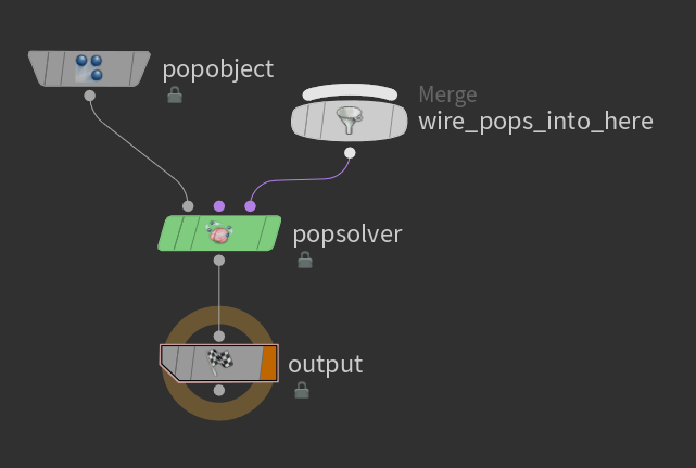
The first thing we need to do is to convert the normal of the sphere into a velocity field. To do that, let's do the following node connections:

We will enable 'pre-compute normals' on the facet node to calculate the normals on the sphere.

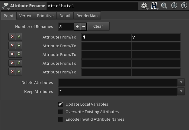
Next let's add a 'attribute rename' node to convert these normals into a velocity field. N represents normals and v represents velocity. Add a null output node after;

Lastly, let's connect a popnet node at the end:

Right away, we get some results.

Let's replace the sphere from above with a tube, and we will get the following result:

Furthermore, we can generate points directly on our emitter geometry and use these points as source of our particles. 

For example, if we add either a 'scatter'  node to generate some points on our geometry (turn off maximum counts, and set relax iterations to 0), inside the popnet, we will simply set the Emission Type to 'all points', and this will utilize all the points on the emitter geometry to emit the particles.

Also with the scatter node, we can manually control the number of points to be scattered on the geometry (which will in turn affect the number of particles emitted) via the force total count parameter.

We will also add a point velocity node to add some noises/randomness to the normal velocity of the emitter geometry.

If we use some VEXpressions on the Impulse Activation, we can make the particles emit in step rather than continuously. If we type an expression like $F%10 == 0, this will activate the particles every 10 frames.

In the birth activation, let's set the VEXpression to $F == 1 so that the particles are emitted once. We are doing this because we want to be able to control the behaviour of the birthed particles. Then later, we will make them emit at intervals. 

Let's set the inherit velocity of the pop source to 20.

Let's also add a ground plane as a collider by connecting a 'ground plane' node to the setup, we will also hide the ground plane geometry. So when we play the simulation, the particles will collide with the ground plane:

Let's add a pop drag and a pop force to the particles. The drag will slow down the movement of the particles after they are emitted, and we will use the pop force to add some disturbance/turbulence to the particles motion.

On the point velocity node, we will set the velocity to 'keep incoming'.

In the curl noise tab, we will enable 'add curl noise' and also 'animated'. Then set the scale and swirl size as well.

This will add more chaos to the generated particles. Let's also reduce the lifespan of the particles to 1, and lifespan variance to 0.5 so that they die quickly.

Since we are trying to create a shockwave, the particles currently spread out in the Z direction too much. Let's use a transform node on the emitter geometry to thin them out. Set the Scale Z to 0.2;

Now, let's increase the particles count and also change the VEXpression back to $F%5==0, we will get the following result for our shockwave:

Let's add a blast node after the popnet, and choose the group in the dropdown and delete non-selected; This will prune out any particles that isn't part of the selected group for us.

We can add another transform node to thin out the particles even further;

We can also crank up the total number of particles to about 500,000;

Right now, we can't really see the pattern of the shockwave field because there isn't much gaps between each particles emission. So let's increase the modulus to 15 in the VEXpression in the Impulse Activation, that is $F%15==0.

Now, each patterns are distinct.

Caching out the particles is pretty easy. It's pretty much the same steps as we have learnt in other types of simulations.

In the geometry SOP level, let's connect a file cache node to the output of the popnet setup, specify an output directory and do the usual naming convention;

After caching, we can use the particle fluid surface node to preview our particles, by changing the convert to to 'particles'.

Then to export to Maya, we simply need to create a Houdini Digital asset using the particles cache files. 

We will have to create a new subnet node in the object level to do this, and then follow the usual steps to export them as HDA (refer to the Houdini-Maya workflow module to learn how to export Houdini particles into Maya).

Below is a viewport and render preview of the particles inside Maya:

We can also choose to render the particles inside Houdini. Let's take a quick look at that.

Let's go back to the object level and change the viewport to Render View. Without doing anything else, if we hit the render button, we will currently have this result:

The particles are currently being rendered as spheres.

Select the geometry node and in the parameter, change the tab to 'Render'. Navigate to the Geometry subtab. We will see that 'Render points as' is currently set to 'Spheres' (Remember that we define particles as points in the 3D space in the beginning).

If we reduce the point scale to say 0.05 and update the render, we will see the spheres size has now reduced and it's starting to feel like shockwaves.

Let's assign some materials to the particles now. So switch to the 'Material Palette' tab, drag and drop the principled shader into the viewer. Then double click on the principled shader to go into it's properties settings.

To assign the materials to the particles, copy the principled shader node, then go back to the object level, select the shockwaves geometry node, and under the render tab, material field, paste the copied material there. It will now be assigned to the particles.

This is basically how you can assign materials to any object inside Houdini. 

Now all we have to do is to tweak the shader till we get our desired result.

To get the look of the shockwave, let's first turn down the albedo color, and set reflectivity to zero. Also, we will choose a blue emission color. 

Under the opacity tab, set it to 0.05 (if we are using emission with opacity, when the opacity is low, it would increase the effect of the emission). 

So we will have something like this in the render now:

Let's enable motion blur. Navigate to the output view in the node editor, under the Rendering subtab, enable 'allow motion blur'.

Let's also back to object level, select the geometry node, and under the rendering sampling tab, we will change it to 'velocity blur'.

Right now, we are getting some pixelations. Let's clean things up. Go back to the OUT view, and under sampling subtab, let's increase Pixel Samples to 10 by 10. We can also reduce the VEXpression on the Impulse activation back to $F%5==0 so that we get a more compact look.

Now we are really starting to get that energy field look. We can use a post-processing tool like aftereffects to add some more motion blur so that we don't see those individual particles like we are seeing here.